mediocreatbest.xyz

Originally posted on Mastodon.

I finally got out of a bit of a depressive lull and funk for coding things for fun, and I was able to make something cute that I think is possibly even useful.

I've been playing with #LLM text #embedding #models.

I've been interested in using them as a tool to filter long lists of text into a shorter list that I can process myself.

Specific example: I wanted to find all recently published papers in a certain topic area from a journal in my field. There's ~300 papers. Only ~10 are relevant.

---

For my first attempt, I hand picked ~5 papers out of ~100 papers. I then used the paper's title, author list, abstract, and keywords to get a text representation of the paper.

I knew that I wanted to try applying Content Defined Chunking to the problem, to split a long text into more manageable pieces.

However, I didn't know the optimal chunking size, so I tried multiple strategies and weighted them by their length.

For instance, chunks of 32 chars at 0.25 weight vs 256 char at 0.75 weight.

---

The result of this experiment is in this Google Colab notebook: https://gist.github.com/player1537/c5970698349ec635c361e92321f2ca1c

I was ultimately able to produce a list of around 40 papers that I should look more closely at. I'm still looking through these, but this is much better than the ~300 I started with.

---

While working on this, I realized that it'd be nice to be able to share a URL to someone of that point in a semantic embedding space.

The challenge: the smallest embedding models yield vectors of size 384. Naively, this can be encoded as a very, very large URL, but not something small enough that a human could feasibly type it themselves.

So, I wondered: could you embed a quantized version of the vector? What quantization would work: 8 bit? smaller? even 1 bit?

---

There's an interesting property that actually makes 1 bit encoding unique.

First, consider that when doing cosine similarity of embedding vectors, you first normalize the incoming vectors, then do a dot product.

Then, consider that encoding 0 bits as negative and 1 bits as positive means that you can use bitwise operators to do the dot product.

I coded that idea: https://gist.github.com/player1537/cf5dc8853ccfe4767660e703d06d6a1e

---

Then, how to encode as a string? Well, we're already comfortable with UUIDs at 128 bits encoded as ~36 hex characters, so encoding 384 bits as ~64 base64 characters isn't much worse.

The encoding process is also in that notebook

The punchline: this method allows you to represent the text “AdaVis: Adaptive and Explainable Visualization Recommendation for Tabular Data” as the embedding:

8eG2V2UQTNVqfa+mG/2zpGRaokJ00yr5b0ww6zybFrzLK2F2XepPCBpseCQnDopE

which is small enough to be manageable imo!

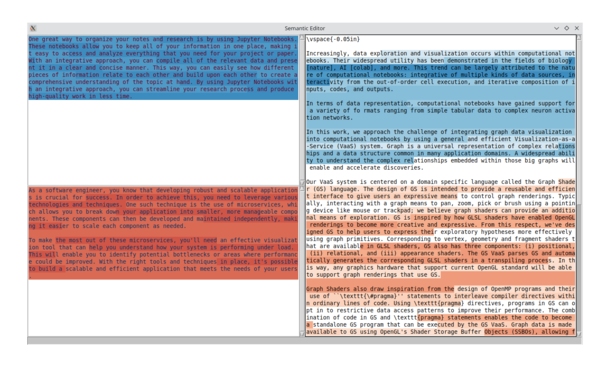
I'd like to share a little tool that I created that I've been playing with. I think now is the time to share it because I believe it has a unique solution to the “how do you chunk up a document” for #LLM #embeddings, which is something @simon@simonwillison.net" title="simon@simonwillison.net">@simon mentioned being an open challenge in his recent blog post.

I've been calling it Semeditor, short for Semantic Editor, available here: https://gist.github.com/player1537/1c23b91b274d2e885be80d5892bac5b7

It can be run with --demo to get the text from the screenshot.

---

This tool is born out of a need of mine: I'm currently editing an academic paper and I'm in charge of revising the story from one concept (web services) to another concept (jupyter extensions). But that's a tricky thing to quantify: how can one know what the text is actually about?

So, I wanted to create a syntax highlighter that highlights the semantic difference between the meanings of the texts.

---

Functionally, the tool takes two samples of text (top-left, bottom-left) and finds a way to differentiate those two samples.Then, it applies that same differentation on a third sample of text (right) and highlights accordingly.

For the semantic meaning of the text, I used the smallest model I could find: BAAI/bge-small-en. For differentating the text, I used a Support Vector Machine (SVM) classifier.

Now, for what I feel is the most interesting part of this tool: the chunking.

Since this is running locally on one's computer, I really don't want to constantly recompute the embeddings, especially as I'm intending this to be an editor, so the edits could be early on in the text and that would ruin naive chunking strategies.

Instead, I used an implementation of Content Defined Chunking (CDC) for Python called FastCDC.

---

The core idea of CDC is to consistently determine chunk boundaries based on the contents of the text. So, in theory, if you edit one part of the text early on, eventually the chunking will re-align itself with previous chunk boundaries.

I believe this works off of a windowed hashing function, so hash(string[i:i+N]) and check if the first few binary digits are zeros, and if so, output a chunk boundary.

You can control the chunking to get arbitrarily small chunks: I use between 32 and 128 chars.

---

To make each chunk more usable, especially in the face of chunk boundaries cutting words in half, I combine three chunks together to compute the actual embeddings from.

In terms of usability, I've already found this useful, at least marginally. I wanted to flex my tkinter knowledge a bit so I created it as a GUI app and I've found the need to add a couple convenience features. First, repeating the exemplars (left) gives better results. Second, asking an LLM to rephrase helps.

---

I'm scared of sharing projects like these because I worry they'll either be completely ignored, or worse, looked down upon. Regardless, I'm hoping to overcome that fear by just sharing it anyways.

Especially now, because I feel the techniques within it will become obsolete soon, but I think it's an interesting enough technique that I want to share it before it becomes obsolete. Maybe it will inspire someone, who knows.

Originally posted on Mastodon

I wanted to collect some of the snippets that I use for writing Dockerfiles. Obviously, there is a lot of nuance in how to structure the Dockerfile and how to build projects, so this isn't meant to cover every possibility, but instead to serve as a starting point that I can share with others.

FROM

A Dockerfile starts from somewhere and that starting point is the argument to the FROM instruction. There's lots of options: all the main Linux operating systems (e.g. Ubuntu, Debian, Fedora, etc) and some more niche operating systems that can optimize Docker image size and speed (e.g. Alpine).

In general, I think Ubuntu is almost always a reasonable starting point. I like to check what the latest release is and then go one version earlier. So, today (Dec 9, 2022), the Ubuntu Wikipedia article Kinetic Kudu 22.10 as the latest, so I would build the Docker image from Jammy Jellyfish 22.04 LTS.

# File: Dockerfile
FROM ubuntu:jammy

Modern Docker makes it really easy to use multiple build steps for your image. Although useful, I think it's unnecessary to use this as a beginner. To use it though, I've found the following setup to be convenient.

# File: Dockerfile
FROM ubuntu:jammy AS base

# install runtime dependencies

FROM base AS deps

# install development and software dependencies
# build and install current project

FROM base AS dist

# copy files from deps image, e.g.
COPY --from=deps /opt/libfoo /opt/libfoo

installing dependencies with apt

Each operating system has its own method of installing packages. For Ubuntu, the following boilerplate can be used and adapted for each package you want to install.

# File: Dockerfile
FROM ubuntu:jammy

# Tell apt that the install is automated and we aren't directly interacting.
# Only needed once.
ENV DEBIAN_FRONTEND=noninteractive

# Always update the apt index and then always remove any package caches.
RUN apt-get update && \
    apt-get install -y \
        build-essential \
        libpng-dev \
    && rm -rf /var/lib/apt/lists/*

getting source code into build

There's two main ways of getting source code into your build: using git to clone repositories during the build and using git to clone repositories before the build. Docker has some capabilities to make the “cloning during the build” step easier, namely the RUN --mount=git option. However, I think it's generally easier to just clone outside before the build step.

To do this, you can use git submodules or any other method of getting the code accessible locally. The main idea is that from your parent repository, you want something that looks like the following.

host$ tree
.
├── .git
└── libfoo
    └── .git

Then in your Dockerfile, you'd want to include a COPY command.

# File: Dockerfile
FROM ubuntu:jammy

# Make /opt directory if it doesn't exist; make /opt/src directory if it doesn't exist; then run all future commands from /opt/src
WORKDIR /opt/src

# Copy the host's entire libfoo directory into /opt/src/libfoo
COPY ./libfoo ./libfoo

building with cmake

I like to use the following snippet for building CMake projects.

# File: Dockerfile
FROM ubuntu:jammy

# Build the source code from "-H"ere
# Write the "-B"uild files here
# For extra paranoia points: remove the build directory afterwards to avoid bloating the image
RUN cmake \
        -H/opt/src/libfoo \
        -B/opt/src/libfoo/build \
        -DCMAKE_INSTALL_PREFIX:PATH=/opt/libfoo \
        -DCMAKE_BUILD_TYPE:STRING=RelWithDebInfo \
    && \
    cmake \
        --build /opt/src/libfoo/build \
        --verbose \
        --parallel \
    && \
    cmake \
        --install /opt/src/libfoo/build \
        --verbose \
    && rm -rf /opt/src/libfoo/build

ENTRYPOINTs and CMDs

Docker lets you configure the entrypoint (normally something like /bin/bash -c) and the default arguments to that entrypoint (normally no arguments, empty). Although tempting and sometimes useful, I don't think a beginner will ever need to mess with these values.

There is one useful usage of ENTRYPOINT and that's when your Docker image is only meant to run a single application ever and if that application isn't your own. For example, ImageMagick could be convenient to use directly from a container (it's not a great example because ImageMagick includes multiple executables: convert, identify, etc).

# File: Dockerfile
# ...
ENTRYPOINT ["convert"]

With that setup, you could replace every normal use of convert in a shell script with docker run -it --rm --mount type=bind,src=$PWD,dst=$PWD my-convert:latest. It's still not great, admittedly.

other things

Some other things that don't fit in better elsewhere.

• In most cases, try not to use mkdir when you could instead use WORKDIR.
• In most cases, don't use multi-stage (multiple FROM) builds.
• It can sometimes be useful to add a custom user for a Docker image. In most cases, I've found it better to leave the Docker image with the default root user, and instead use your own user when running. For example: docker run -u $(id -u):$(id -g) ...
• I haven't found a good use for the VOLUME command in most of my work. In theory, it's good to document what things can and should be mounted to the host filesystem, but it's rare that that affects me.
• Likewise, EXPOSE is good for documentation but I don't find it that useful.

I ran into a problem when I tried to debug some C++ code that uses VTK. The problem ultimately came down to GDB not understanding that some arguments were being passed via registers instead of on the stack. I worked around this problem using the GDB convenience variable $_caller_is.

Code Example

/**
 *
 */

// stdlib
#include <cstdio>

// VTK
#include <vtkSetGet.h>
#include <vtkObject.h>
#include <vtkNew.h>
#include <vtkObjectFactory.h>


//--- Define a simple vtkObject subclass with the offending method.

struct Foo : public vtkObject {
    static Foo *New();

    vtkSetVector6Macro(Bounds, float);
    float Bounds[6];
};

vtkStandardNewMacro(Foo);


//--- Demonstrate the bug.

int main() {
    vtkNew<Foo> foo;

    float bounds[6];
    bounds[0] = 0.373737f;
    bounds[1] = 1.373737f;
    bounds[2] = 2.373737f;
    bounds[3] = 3.373737f;
    bounds[4] = 4.373737f;
    bounds[5] = 5.373737f;

    std::fprintf(stderr, "main.bounds = { %+0.2f, %+0.2f, %+0.2f, %+0.2f, %+0.2f, %+0.2f };\n",
        bounds[0], bounds[1], bounds[2], bounds[3], bounds[4], bounds[5]);

    foo->SetBounds(bounds);

    std::fprintf(stderr, "foo.Bounds = { %+0.2f, %+0.2f, %+0.2f, %+0.2f, %+0.2f, %+0.2f };\n",
        foo->Bounds[0], foo->Bounds[1], foo->Bounds[2], foo->Bounds[3], foo->Bounds[4], foo->Bounds[5]);

    return 0;
}

My code looked very similar to this. I attached a debugger to it and ran the following gdb batch file.

#!/usr/bin/env -S gdb -x
start
break -function Foo::SetBounds
commands
  printf "---8<---\n"
  info args
  printf "--->8---\n"
  continue
end
continue

What I saw when I ran this was that the first SetBounds call was called with the correct argument, a pointer to a float array with the correct contents. But in the second SetBounds call, I was getting garbage floating point values with extreme exponents (e-41, e21, etc).

To elaborate: in VTK's vtkSetGet.h header, the vtkSetVector6Macro is defined, roughly, as:

#define vtkSetVector6Macro(Name, Type) \
  void Set##Name(const Type *_arg) { \
    this->Set##Name(_arg[0], _arg[1], _arg[2], _arg[3], _arg[4], _arg[5]); \
  } \
  void Set##Name(Type _arg1, Type _arg2, Type _arg3, Type _arg4, Type _arg5) { \
    this->Name[0] = _arg1; \
    this->Name[1] = _arg2; \
    this->Name[2] = _arg3; \
    this->Name[3] = _arg4; \
    this->Name[4] = _arg5; \
    this->Name[5] = _arg6; \
  }

In other words, one function takes a pointer to an array of a type, and the other takes each argument individually. The first function defers to the second to actually update the member variable.

Diagnosing the Problem

I'd already suspected that this could have been a “register vs stack” problem. For this reason, I checked the disassembly of each SetBounds function and saw that it was writing to the %xmm1, %xmm2, etc registers in the first SetBounds function and then reading from %ymm1, %ymm2, etc registers in the second SetBounds function.

Aside: I was a little confused on the switch between %xmm1 and %ymm1. I read online that these are SSE registers that hold multiple floats, chars, etc within a single register. The %xmm1 register holds 4 floats, while the %ymm1 register holds 8 floats, with the first 4 being mirrored in %xmm1.

To verify this, I set a breakpoint in the second SetBounds function, verified that info args showed the incorrect garbage values, and then verified that the %ymm1 register output by info all-registers had the correct values.

Working Around the Problem

Ideally, in GDB, I'd have a way to set a breakpoint on only one of the SetBounds functions. Barring that, I can check if the function that called us is also SetBounds or not (i.e. if we're the second or first, respectively). In a GDB script, that looks like:

#!/usr/bin/env -S gdb -x
start
break -function Foo::SetBounds if ! $_caller_is("Foo::SetBounds")
commands
    printf "Foo::SetBounds((float[6])"
  output *(float *)_arg@6
  printf ")\n"
  continue
end
continue

Scientific code should be compiled and tuned to best match their processor architecture. Some processors have special instructions for maximum performance; for instance, Intel has SSE instructions, and AMD has their specific instructions too. Code compiled for one architecture doesn't necessarily run on another which is the root of the problem.

The primary symptom you would see is a segfault error of an illegal instruction.

29 Illegal instruction     (core dumped)

This is especially prevalent in building and using Linux Containers for HPC systems. On these systems, although you can use container images that have already been built, creating new container images is more challenging because you have to build them separately and then load them onto the HPC system.

For example, I build some of our container images on my server and then use them on one of several supercomputers. For most systems, this is fine because they both happened to be Intel Broadwell chips, but now one of the machines is AMD k10 based. In cross-compiling for the other machine, I ran into a few hiccups, which is what this post is about.

Case Study: Spack

Spack is a tool to help build and manage dependencies for HPC systems. It makes things relatively easy because it allows you to specify the target architecture directly.

First, you can use spack arch to determine what it believes your architecture is on the target machine. In my case, this yielded a value linux-scientific7-k10, according to the triplet platform-os-target (Architecture Specifiers). The most important value is the target.

Next, you can change your spack install command to specify that target. For instance:

$ spack install mpich target=k10

In the case that you're using a spack.yaml configuration file, you can add the packages subtree and specify your target under packages > all > target (Concretization Preferences).

spack:
  specs:
  - mpich
  packages:
    all:
      target: [k10]

One last thing you can do is find the -march and -mtune parameters to use for other cross-compiling endeavors. The easiest way to do this is to check the source code (microarchitectures.json) for your target. For k10, this entry looks like:

{
    // ...
    "k10": {
      "from": "x86_64",
      "vendor": "AuthenticAMD",
      "features": [
        // ...
      ],
      "compilers": {
        "gcc": {
          "name": "amdfam10",
          "versions": "4.3:",
          "flags": "-march={name} -mtune={name}"
        },
        // ...
      }
    },
    // ...
}

Based on the compilers > gcc subtree, we can see that -march=amdfam10 and -mtune=amdfam10. As well, if these weren't specified, we could also check x86_64 for its fields.

Case Study: Python

Python makes it relatively easy to change the compiler target, at least using pip. For this, you need to set the CFLAGS environment variable before installing dependencies (StackOverflow answer that references this).

In my case, I already had the -march and -mtune flags I needed, so I just had to run:

$ CFLAGS='-march=amdfam10 -mtune=amdfam10' \
>   python3 -m pip install networkx

Case Study: Rivet

Rivet is a suite of libraries for particle physics simulation and analysis. For end-users, it is compiled using a bootstrap script, which internally calls into the Rivet libraries' autotools configure script.

To tell autotools what architecture to build for, there are some options like --build, --host, and --target which are all a little confusing. They each require a triple of cpu-company-system (System Type – Autoconf). In general, you can ignore --build and --target for most regular libraries, only using them when compiling compilers (Specifying Target Triplets). To make things easier, you can use shorter names for your architecture and a script will normalize them (gcc/config.sub).

In my case, I wasn't able to find out exactly what name should be used for my target architecture, while I did already know what -march and -mtune names I wanted. So, instead, I found that you can just pass CFLAGS directly to the configure script and it will do the right thing (GitHub issue that references this feature).

$ ./configure CFLAGS='-march=amdfam10 -mtune=amdfam10'
$ make
$ make install

Also, the Rivet bootstrap script doesn't expose a way to give the configure scripts any extra arguments. Instead, it uses a function that just passes an install prefix along. The replacement is as follows:

# before
function conf { ./configure --prefix=$INSTALL_PREFIX "$@"; }

# after
function conf {
  ./configure --march=amdfam10 --mtune=amdfam10 --prefix=$INSTALL_PREFIX "$@"
}

I had written up a few posts before, but it wasn't working for me. Now with this WriteFreely blog, I'm hoping to write more. Regardless, the old posts are still available:

old posts